Pointwise bootstrap intervals
What this example reviews
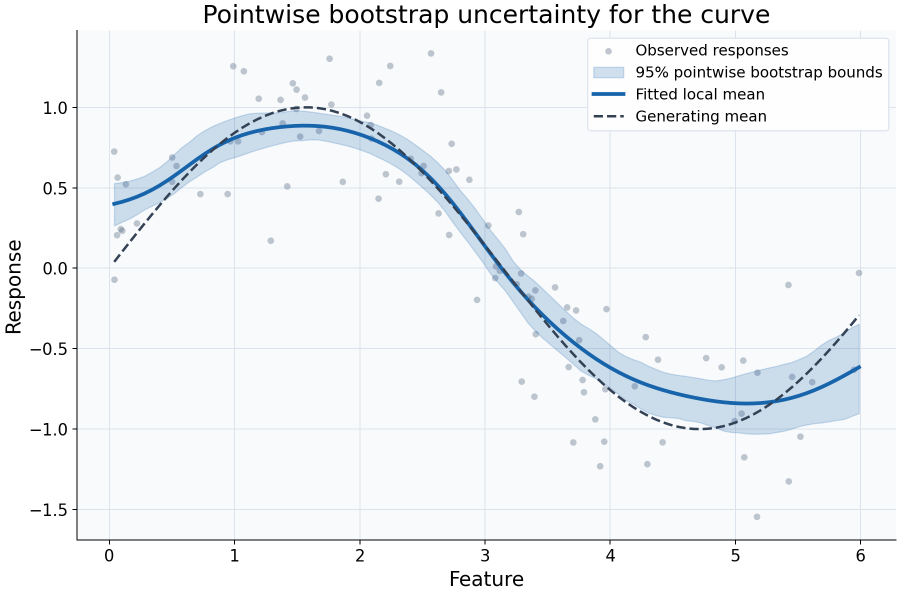
This example reviews sampling uncertainty around a fitted regression curve. Independent synthetic feature values are sampled uniformly, then explicitly sorted before independent response noise is generated. A Gaussian local-constant fit uses bandwidth 0.4. Paired IID bootstrap resampling refits the model and evaluates bounds at 100 locations in the original observed feature range.
Choices and their impact
| Item | What is being reviewed | Impact and interpretation |
|---|---|---|
| Gray responses | Variation of individual observations | Their vertical spread is response noise, which is not the target of the shaded curve intervals. |
| Blue fitted curve | The local response mean estimated from the original data | Remains the reference estimate while the bootstrap describes variation across resampled fits. |
| Shaded 95% bounds | Pointwise percentile bootstrap intervals | At each query, bounds come from the distribution of bootstrap predictions. Connecting them is a display choice, not a simultaneous band. |
| Dashed generating mean | Known synthetic relationship | Makes possible smoothing bias visible; the bootstrap does not correct that bias. |
| 100 resamples and fixed seed | Monte Carlo calculation and reproducibility | The seed makes this run reproducible. More draws improve numerical stability of bootstrap quantiles, not the validity of sampling assumptions. |
| 100 query locations | Where uncertainty is evaluated | More locations increase plotting detail and computation without adding training data. |
Interpreting the plot
Read the shaded region as uncertainty about a fitted curve at each separate location. It is not the expected spread of a future response and does not imply 95% coverage of the entire curve at once. Compare the original fit with the dashed mean as well as with its bounds: systematic smoothing bias may remain even when bounds look narrow.
Inspect n_valid and bootstrap_coverage before interpreting a bound. They count
finite bootstrap predictions, rather than estimating nominal confidence coverage.
The default requires every draw to support a query; otherwise bounds remain NaN.
Resampled feature ranges may differ from the original range, so extrapolation
advisories can occur during this example even though the original queries are in range.
When this is useful
Use this workflow to explore how sensitive a curve statistic is to sampling and to communicate its pointwise bootstrap variability. It is more informative than drawing a response-spread envelope and calling it uncertainty about the mean.
Paired IID resampling assumes independent random-design rows. Grouped or ordered dependent observations need appropriate resampling choices. The selected bandwidth is held fixed: these bounds omit bandwidth-selection uncertainty and smoothing-bias correction. They do not remove confounding or certify extrapolation.
Explore further
Increase n_resamples, retaining the seed and data, to examine Monte Carlo
stability. Change confidence_level to compare nominal interval levels. For a
suitable dependent dataset, investigate group/block resampling rather than
interpreting IID bounds as universally valid.
Run this example
From the checkout, with rgram[plot] installed:
python examples/plot_relationships.py --example intervals
# Save just this figure without opening a desktop window:
python examples/plot_relationships.py --example intervals --output-dir /tmp/rgram-figures
Download this standalone example.
The complete code below includes imports, data, configuration, and plotting.
Run the downloaded file with python intervals.py.
from __future__ import annotations

import argparse
from pathlib import Path
from typing import TYPE_CHECKING
import warnings

import numpy as np

from rgram import KernelSmoother, Regressogram, SupportWarning, quantile

if TYPE_CHECKING:
    from matplotlib.axes import Axes
    from matplotlib.figure import Figure

# A consistent palette makes comparisons readable across the gallery.
COLORS = ["#1764ab", "#de682b", "#21856b", "#8855a2"]


def _create_axes(
    title: str, xlabel: str = "Feature", ylabel: str = "Response"
) -> tuple[Figure, Axes]:
    """Create a readable, single-panel figure with consistent gallery styling."""
    import matplotlib.pyplot as plt

    with plt.rc_context({"font.size": 14, "axes.labelsize": 16, "axes.titlesize": 20}):
        figure, ax = plt.subplots(figsize=(10, 6.6), layout="constrained")
        ax.set(title=title, xlabel=xlabel, ylabel=ylabel)
    ax.set_facecolor("#f8fafc")
    ax.grid(color="#dce3ec", linewidth=0.8)
    ax.set_axisbelow(True)
    ax.spines[["top", "right"]].set_visible(False)
    ax.tick_params(labelsize=13)
    return figure, ax


def _plot_observations(ax: Axes, X: np.ndarray, y: np.ndarray) -> None:
    """Show original rows without connecting them or hiding response spread."""
    ax.scatter(
        X,
        y,
        color="#64748b",
        alpha=0.4,
        s=28,
        edgecolors="none",
        label="Observed responses",
    )


def _add_legend(ax: Axes) -> None:
    """Identify every plotted comparison using the same readable legend style."""
    ax.legend(fontsize=12, framealpha=0.96, edgecolor="#dce3ec", loc="best")


def _gaussian_smoother(bandwidth: float, **kwargs) -> KernelSmoother:
    """Keep kernel and bandwidth units explicit; kwargs select other model options."""
    return KernelSmoother(
        kernel="gaussian", bandwidth="manual", bandwidth_value=bandwidth, **kwargs
    )


def intervals() -> Figure:
    """Display supported pointwise bootstrap bounds for a regression curve."""
    rng = np.random.default_rng(17)
    # Sample a random design with independent noise, appropriate to paired IID draws.
    # Sorting is explicit here for the display; the estimator never sorts rows.
    X = np.sort(rng.uniform(0, 6, 100))
    y = np.sin(X) + rng.normal(0, 0.3, len(X))
    # Keep original queries in the observed range; resampled ranges can differ.
    query = np.linspace(X.min(), X.max(), 100)
    model = _gaussian_smoother(0.4).fit(X, y)
    # Fix the seed for reproducibility. More draws reduce Monte Carlo variation,
    # but do not correct smoothing bias or include bandwidth-selection uncertainty.
    interval = model.predict_interval(query, n_resamples=100, random_state=17)
    figure, ax = _create_axes("Pointwise bootstrap uncertainty for the curve")
    _plot_observations(ax, X, y)
    # Connecting pointwise bounds is a display choice, not a simultaneous band.
    # NaN bounds would remain gaps rather than being silently filled.
    ax.fill_between(
        query,
        interval["lower"].to_numpy(),
        interval["upper"].to_numpy(),
        color=COLORS[0],
        alpha=0.2,
        label="95% pointwise bootstrap bounds",
    )
    ax.plot(
        query,
        interval["prediction"].to_numpy(),
        color=COLORS[0],
        lw=3,
        label="Fitted local mean",
    )
    ax.plot(query, np.sin(query), "--", color="#334155", lw=2, label="Generating mean")
    _add_legend(ax)
    return figure

if __name__ == "__main__":
    import matplotlib.pyplot as plt

    figure = intervals()
    plt.show()
    plt.close(figure)